1 RCircos plot with human genomic data

Authors: Hongen Zhang  Reviser: Tianze Cao

2025-06-04

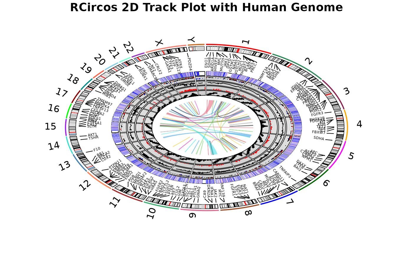
This demo draw human chromosome ideogram and data tracks for:

1. Connectors
2. Gene lables
3. Heatmap
4. Scatterplot
5. Line plot
6. Histogram
7. Tile plot
8. Link lines

# Load RCircos package

library(RCircos);

# Load human cytoband data

data(UCSC.HG19.Human.CytoBandIdeogram);
hg19.cyto <- UCSC.HG19.Human.CytoBandIdeogram;

# Setup RCircos core components:

RCircos.Set.Core.Components(cyto.info=hg19.cyto, chr.exclude=NULL, tracks.inside=10, tracks.outside=0);

## 
## RCircos.Core.Components initialized.
## Type ?RCircos.Reset.Plot.Parameters to see how to modify the core components.

# Open the graphic device (here a pdf file)

message("Open graphic device and start plot ...\n");

## Open graphic device and start plot ...

RCircos.Set.Plot.Area();
title("RCircos 2D Track Plot with Human Genome");

# Draw chromosome ideogram

message("Draw chromosome ideogram ...\n");

## Draw chromosome ideogram ...

RCircos.Chromosome.Ideogram.Plot();

# Connectors in first track and gene names in the second track.

message("Add Gene and connector tracks ...\n");

## Add Gene and connector tracks ...

data(RCircos.Gene.Label.Data);

RCircos.Gene.Connector.Plot(genomic.data=RCircos.Gene.Label.Data, track.num=1, side="in");

## Not all labels will be plotted.

## Type RCircos.Get.Gene.Name.Plot.Parameters()

## to see the number of labels for each chromosome.

RCircos.Gene.Name.Plot(gene.data=RCircos.Gene.Label.Data, name.col=4,  track.num=2, side="in");

## Not all labels will be plotted.

## Type RCircos.Get.Gene.Name.Plot.Parameters()

## to see the number of labels for each chromosome.

# Heatmap plot. Since some gene names plotted above are longer than one track height, we skip two tracks

message("Add heatmap track ...\n");

## Add heatmap track ...

data(RCircos.Heatmap.Data);
RCircos.Heatmap.Plot(heatmap.data=RCircos.Heatmap.Data, data.col=6, track.num=5, side="in");

# Scatterplot. Note: There is no prefix of "chr" in chromosome names of RCircos.Scatter.Data

message("Add scatterplot track ...\n");

## Add scatterplot track ...

data(RCircos.Scatter.Data);
RCircos.Scatter.Plot(scatter.data=RCircos.Scatter.Data, data.col=5, track.num=6, side="in", by.fold=1);

# Line plot. Note: There is no prefix of "chr" in chromosome names of RCircos.Line.Data

message("Add line plot track ...\n");

## Add line plot track ...

data(RCircos.Line.Data);
RCircos.Line.Data[,1] <- paste0("chr", RCircos.Line.Data[,1])
RCircos.Line.Plot(line.data=RCircos.Line.Data, data.col=5, track.num=7, side="in");

# Histogram plot

message("Add histogram track ...\n");

## Add histogram track ...

data(RCircos.Histogram.Data);
RCircos.Histogram.Plot(hist.data=RCircos.Histogram.Data, data.col=4, 
             track.num=8, side="in");

# Tile plot. Note: tile plot data have chromosome locations and each data file is for one track

message("Add tile track ...\n");

## Add tile track ...

data(RCircos.Tile.Data);
RCircos.Tile.Plot(tile.data=RCircos.Tile.Data, track.num=9, side="in");

## Tiles plot may use more than one track. Please select correct area for next track if necessary.

# Link lines. Link data has only paired chromosome locations in each row and link lines are always drawn inside of chromosome ideogram.

message("Add link track ...\n");

## Add link track ...

data(RCircos.Link.Data);
RCircos.Link.Plot(link.data=RCircos.Link.Data, track.num=11, 
             by.chromosome=FALSE);

# Add ribbon link to the center of plot area (link lines).

message("Add ribbons to link track ...\n");

## Add ribbons to link track ...

data(RCircos.Ribbon.Data);
RCircos.Ribbon.Plot(ribbon.data=RCircos.Ribbon.Data, track.num=11, 
             by.chromosome=FALSE, twist=FALSE);